Cloud work doesn’t start with services. It starts with the account.
Before deploying any workloads, I focused on establishing a secure, enterprise-ready AWS foundation aligned with real-world production standards.
Key areas addressed:
 AWS Account Security & Governance
Root account lockdown (MFA, no access keys, billing controls)
Cost monitoring and budget alerts from day one
 IAM & Access Management (Best Practices)
Role-based access control (RBAC) using IAM roles
Elimination of standing admin privileges
MFA enforced for all human access
 AWS IAM Identity Center (SSO)
Centralized identity and authentication
Permission sets instead of ad-hoc IAM policies
Temporary credentials aligned with AWS Organizations and SCP-ready patterns
茶 Auditability, Compliance & Threat Detection
CloudTrail enabled across all regions for API auditing
AWS Config for configuration and change tracking
GuardDuty for continuous threat detection
Outcome:
An AWS account that is secure, observable, auditable, and scalable before any workloads are introduced — the same baseline expected in regulated and production environments.
This kind of foundation reduces security risk, accelerates future delivery, and prevents painful rework later.
Cloud maturity isn’t about spinning up resources fast.
It’s about governance, security, and intent from day one.

Partition Pruning
Your WHERE clause isn’t helping—here’s why Snowflake scans everything anyway
I watched a query scan 500GB of data when it should have touched less than 5GB. Same WHERE clause. Same filter. The problem? Snowflake couldn’t prune partitions effectively.
This cost us hours of runtime and thousands in credits—until we understood what was actually happening.
The micro-partition problem:
Snowflake automatically divides tables into micro-partitions (typically 50-500MB compressed). Each micro-partition stores metadata about the min/max values it contains for every column.
When you run a query with a WHERE clause, Snowflake checks this metadata to skip partitions that couldn’t possibly contain your data. This is partition pruning—and when it works, it’s magic.
But here’s the catch: pruning only works if your data is naturally ordered in a way that aligns with your filters.
When I’ve seen this break:
Working with large subscription and order tables, we’d filter by order_date constantly. Sounds perfect for pruning, right?
Except our data wasn’t loaded chronologically. Orders came in from multiple sources, backfills happened, late-arriving data got appended. The result? Every micro-partition contained a mix of dates spanning months.
Query: WHERE order_date = ‘2024-01-15’
Snowflake’s response: “Well, that date MIGHT be in any of these 10,000 partitions, so I’ll scan them all.”
The clustering key solution:
We added a clustering key on order_date for our largest tables:
ALTER TABLE orders CLUSTER BY (order_date);
Snowflake reorganizes data so that rows with similar values are stored together. Now each micro-partition contains a narrow date range, and pruning actually works.
Same query. 5GB scanned instead of 500GB. 95% improvement.
How to check if you’re pruning effectively:
Run your query and check the query profile. Look for “Partitions scanned” vs “Partitions total”:
— Your actual query
SELECT *
FROM orders
WHERE order_date = ‘2024-01-15’;

— Then check the profile or run:
SELECT
    query_id,
    partitions_scanned,
    partitions_total,
    bytes_scanned,
    (partitions_scanned::float / partitions_total) * 100 as scan_percentage
FROM TABLE(INFORMATION_SCHEMA.QUERY_HISTORY())
WHERE query_id = LAST_QUERY_ID();
What to look for:
Scanning >25% of partitions? Probably not pruning well
Scanning <10%? Good pruning
Scanning 100%? No pruning at all
Common culprits:
→ Filtering on columns with random distribution (UUIDs, hashed values)
→ Using functions in WHERE clauses: WHERE DATE(timestamp_col) = … prevents pruning
→ Data loaded out of order without clustering
→ OR conditions across multiple high-cardinality columns
My decision framework for clustering:
Cluster when:
Table is large (multi-TB)
You filter/join on specific columns repeatedly
Query profiles show poor pruning
The column has natural ordering (dates, sequential IDs)
Don’t cluster when:
Table is small (<100GB)
Query patterns vary wildly
Clustering would cost more than it saves (maintenance overhead)
High-cardinality columns with random distribution
The real cost of bad pruning:
It’s not just slower queries. You’re paying to scan data you’ll immediately discard. Every GB scanned consumes credits, even if filtered out.
For our daily reporting jobs on clustered tables, we saw 60-70% reductions in both runtime and credit consumption. The clustering maintenance cost? Negligible compared to the savings.
Quick win you can try today:
Check your largest, most-queried tables. Run your common WHERE clause patterns. Look at partition scan ratios.
If you’re scanning >50% of partitions on filtered queries, you’ve found your optimization opportunity.
What’s been your experience with partition pruning? Have you seen dramatic improvements from clustering?
#Snowflake #DataEngineering #PerformanceOptimization #CostOptimization

ISO/IEC has released several versions of the (ANSI) SQL standard. Each is a list of requirements adopted by representatives from industry in 60 countries. ANSI, the American National Standards Institute, is the official U.S. representative to ISO. The SQL standards are implemented in varying degrees in subsequent releases from major database platform vendors.

The major vendors benefit from the standard because it partially completes requirements gathering for future releases. Their products are made of interpretations and compromises built on prior interpretation and compromise. Marketing is a factor driving adoption of standards. Why prioritize standards customers haven’t asked for?

Then there are the “disruptive innovators.” In the world of database this usually means that either: a paper critical of a standard or a vendor implementation of a standard launched a startup.  Popular disruptions often find their way into the major vendor’s products.

These disruptors have been branded NoSQL and BigData. NoSQL offered document store, graph, key-value, and object databases to name a few. BigData offered relaxed concurrency for high volume high speed data. Most of these functionalities have already been included in recent release from the major vendors.

The major vendors of database platforms are IBM, Microsoft, Oracle, and SAP. IBM has DB2. Microsoft has SQL Server and Azure SQL. Oracle has Oracle, as well as MySQL which they acquired with Sun Microsystems. And SAP has SAP HANA.

These vendors offer a whole host of products in the ERP, CRM, HRM, DSS, and Analytics spaces (to name a few) most of which require a database). There are third party vendors offering Enterprise Resource Planning (ERP), Customer Relationship Management (CRM), Human Resources Management (HRM), Decision Support Systems (DSS) and Analytics Systems each of which will have some degree of preference for one of the major vendors.

What is done with data and with which software drives adoption. This is marketing engineering. Other factors that contribute to adoption is compatibility. Until recently Microsoft’s SQL Server did not run on Linux, but most every other major vendor’s software ran on both Linux and Windows. Licensing can also affect adoption. SQL Server is popular in part because of the ubiquity of Windows and Microsoft Office, each of which contribute to volume licensing requirements that lower the cost of software and support.

In my humble opinion, SQL Server, Oracle, and IBM DB2 are the best documented. Documentation should be a driver in adoption. A poorly documented system is one that is destined to fail miserably.

SQL stands for Structured Query Language. Some people prefer to spell it out, S-Q-L, others pronounce it sequel [ˈsēkwəl]. SQL is a standard defined and maintained by the American National Standards Institute (ANSI) as well as International Organization for Standards – International Electrotechnical Commission (ISO/EIC). It comes in numerous variants. These are specific to database systems that implement the standard. There are also numerous SQL like languages.

You should care about SQL if you care about data. SQL primarily functions to describe tables of data. It instructs the database system to create, modify, or retrieve some form of table. Is it possible to write SQL that in no way describes a table? Feel free to find and share cases that don’t fit neatly into “tables”?

Understanding tables will help you understand how you can use SQL. SQL has the keywords CREATE, ALTER, and DROP which can be used to make, change, and destroy tables. These keywords can make other objects like functions, stored procedures, and views (users, logins, triggers, audits, connections, … etc.). While technically not tables, they do exist as rows in tables. These keywords can also be used to make indexes which help table operations be performed more efficiently.

Often, a person will be working with tables that already exist. In these cases, the SQL keywords SELECT, INSERT, UPDATE and DELETE will be used to perform CRUD operations. CRUD stands for Create, Read, Update, and Delete. These operations are often being performed by multiple users simultaneously.

Multi-user access is an important consideration. The SQL standard prescribes Isolation Levels. These are approaches to the problems that happen with multiple user simultaneous access. These contribute to ACID compliance. ACID stands for Atomicity, Consistency, Isolation and Durability. This is what a lot of “NoSQL” languages tend to do without. Without it, it’s a fast paced free for all that can leave a mess. With it deadlocking and blocking can occur.

These issues shouldn’t stop a data user from becoming an SQL Pro. They just mean you should consult a SQL Pro with experience and keep focused on what matters. SQL itself is by design simple and intuitive (maybe).

SQL is declarative. A user need not know how to create locks or latches, nor which algorithms most efficiently sort, sample, or join. SQL allows the user to declare the state they wish data to be in. The database platform determines based on the structures in play, the statistics available, and other factors how best to fill the request.

When operations are performed the database uses a state transformation known as a transaction. In short, a transaction is an all or nothing operation. It allows multiple tables to be either a start or finish state. Transactions are self-contained. The state is either as it was or as it was intended. Transactions operate independent of other transactions. They are permanent once completed.

In short SQL is a language for working with data in database systems. SQL allows you to describe what you want and get it. It allows a whole host of technical issues to be left to software engineers, database architects and administrators.

If you are asking yourself that, you are administering SQL Server 2016 network or services for the first time, or found some dusty old instance that should be decommissioned. In the latter case you are looking for Enterprise Manager, and perhaps someone to accept responsibility for the change control request.

In the case of 2016 you may not have noticed but its where it has always been.

“What? No it’s not. I looked in the SQL Server folder of the start menu.” you say.

Ok. It’s not there but it is still a snap-in for Microsoft Management Console (MMC).

If you never knew that there was a such thing as MMC, you only need a few quick steps to get up and running.

First, you press the Windows key on you keyboard. If you are unfortunate enough to not have one of those you click the start menu.

Next you type MMC. If you notice that a familiar little icon of a toolbox on a window didn’t appear but instead it you highlighted something starting with the letter M, then something else, then perhaps something starting with a C, you might want to think about Windows end of support dates. For now, click run, and then type MMC.

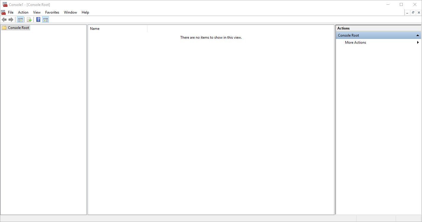
In either case you should be able to launch the MMC.exe console.

Unless, someone configured it for you, the console is going to be this rather uninteresting window:

If you open the file menu and select add/remove snap-in…. (CTRL+M for keyboardists), you will be presented with the Add or Remove Snap-ins dialog.

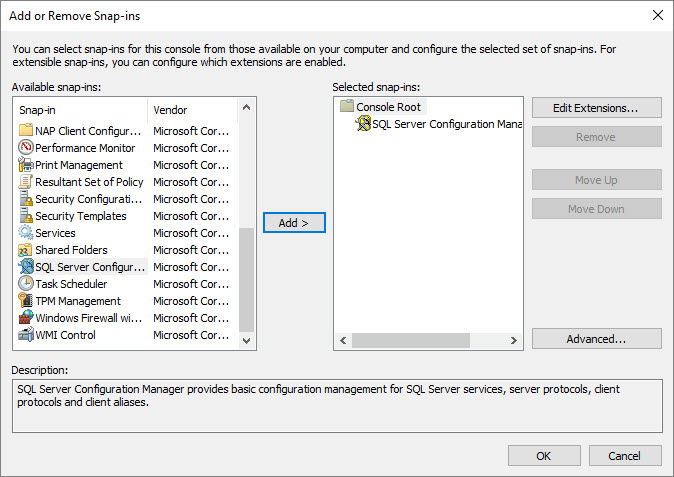
From there you can scroll down to SQL Server Configuration Manager. Click add. Click Ok. And now you have SQL Server Configuration Manager.

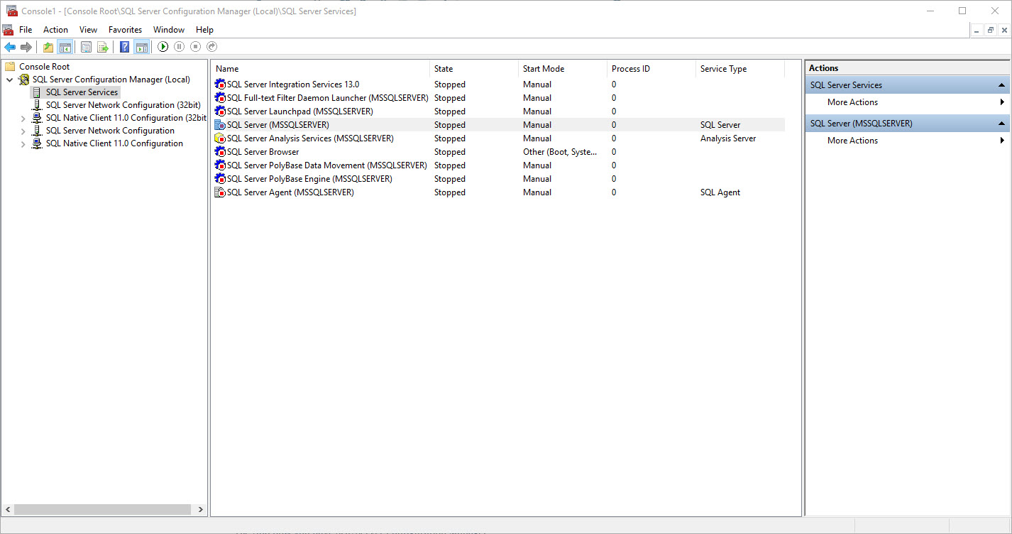
As you may have guessed you can add other useful snap-ins  like (Performance Monitor, Disk Management, Event Viewer, Services, WMI Control, ADUC, RSAT, or Computer/Server Management).

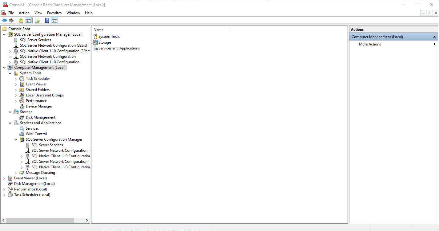
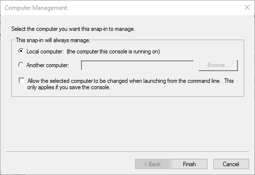
In case you missed it, while we were adding all those cool snap-ins most of which are  part of Computer/Server Management, you can select the local computer or a remote server.

If you like that you can save the console and give it a name. You can also configure folders to hold different groups of servers. You can also create favorites and organize the relationships between the snap-ins to allow you to drill down through common troubleshooting steps. For example you might like to see a performance monitor snap-in configured to view IO related counters as a child of disk management.

MMC is great tool. Now you have to use it. Try and enjoy.

SQL Server 2016 and Azure SQL Database implement a new feature called Temporal Tables, not to be confused with Temporary Tables. This feature implements in a common sense fashion the needs of database applications to maintain a history of changes not just for auditing but for the purpose of analytics.

Temporal Tables allow a user to leverage the FOR SYSTEM_TIME clause when querying a table which was created with the SYSTEM_VERSIONING = ON. Users can also query the temporal history table directly, which is necessary for history values with a duration of zero (e.g. rows updated multiple times in a single transaction).

In honor of Super Bowl 50 I put together a quick visualization with Power Map in Excel 2016. We can see the scores of each team by the size of the dot on their cities. We can also see the number of people in attendance as the height of the bar on the hosting city.

Yesterday, working with a colleague the topic got steered towards the use of snippets in SQL Server 2012+. My reflex was to let my colleague know that my blog is wonderful source for all things SQL Server. Much to my chagrin, for all of the snippets I have, I have written a blog post about it.

Visual Studio has had code snippets for a decade now, but SQL Server only got them a version and a half ago. I might imagine that having templates was the excuse given for not pursuing them but I am glad we have them now. The tools menu will lead you to the Code Snippets Manager… from there you can find the path to built-in snippets. These provide good fodder for creating your own.

There are two types of snippets. Expansion snippets insert the code snippet where the cursor is. Surround snippets wrap code around highlighted SQL. Both have arguments that allow you to tab through variable portions and update multiple references in a single place. Let’s take a look at a simple expansion snippet.

<?xml version="1.0" encoding="utf-8" ?>
<CodeSnippets  xmlns="http://schemas.microsoft.com/VisualStudio/2005/CodeSnippet">
<_locDefinition xmlns="urn:locstudio">
    <_locDefault _loc="locNone" />
    <_locTag _loc="locData">Title</_locTag>
    <_locTag _loc="locData">Description</_locTag>
    <_locTag _loc="locData">Author</_locTag>
    <_locTag _loc="locData">ToolTip</_locTag>
</_locDefinition>
	<CodeSnippet Format="1.0.0">
		<Header>
			<Title>Create Temporary Table</Title>
			<Shortcut></Shortcut>
			<Description>Creates a temporary table.</Description>
			<Author>Thomas W Marshall</Author>
			<SnippetTypes>
				<SnippetType>Expansion</SnippetType>
			</SnippetTypes>
		</Header>
		<Snippet>
			<Declarations>
                                <Literal>
                                	<ID>TableName</ID>
                                	<ToolTip>Name of the Table</ToolTip>
                                	<Default>TableName</Default>
                                </Literal>
                                <Literal>
                                	<ID>Column1</ID>
                                	<ToolTip>Name of the Columneter</ToolTip>
                                	<Default>Column1</Default>
                                </Literal>
                                <Literal>
                                	<ID>Datatype_Column1</ID>
                                	<ToolTip>Data type of the Columneter</ToolTip>
                                	<Default>int</Default>
                                </Literal>
                                <Literal>
                                	<ID>Column2</ID>
                                	<ToolTip>Name of the Column</ToolTip>
                                	<Default>Column2</Default>
                                </Literal>
                                <Literal>
                                	<ID>Datatype_Column2</ID>
                                	<ToolTip>Data type of the Column </ToolTip>
                                	<Default>char(5)</Default>
                                </Literal>
			</Declarations>
			<Code Language="SQL"><![CDATA[

IF EXISTS(SELECT name FROM tempdb.sys.objects WHERE object_id=OBJECT_ID('tempdb..#$TableName$') AND type = N'U') DROP TABLE #$TableName$;
CREATE TABLE #$TableName$
(
    $Column1$ $Datatype_Column1$,
    $Column2$ $Datatype_Column2$
);

]]>
			</Code>
		</Snippet>
	</CodeSnippet>
</CodeSnippets>

You can copy the above XML into a file with the extension .snippet and save it in the Code Snippets\SQL\My Code Snippets directory. You should then see it in the Code Snippets manager. Alternatively, you can import a .snippet file using the Code Snippets manager. Once the snippet has been installed whenever you strike the expansion chord CTRL+K,X in SQL Server Management Studio you will see it in the My Code Snippets folder of the fly-out menu.

In the above XML document we can see a field in the declarations for each of the variable fields. Once you have chosen to insert the snippet those declare fields are linked by there name appearing between $’s. This allows you to change the value in one and have all instances of that name update. You can also tab to the next name.